Isogeometric analysis

Our main mathematical tool to model alpine ski is known as isogeometric analysis (IGA), which is basically an extension of the finite element method (FEM) using non-uniform rational B-splines (NURBS) as basis functions. Being introduced in 2005 by Hughes et al., followed by a book in 2009, IGA tries to bridge the gap between finite element analysis and CAD design tools. The important future of IGA is that it uses the same basis as CAD software for describing the given geometry, and thus exact representation of the model is possible. It is therefore natural to include a section considering this basis in the beginning before we set up the IGA. Note that only the relevant parts of the IGA will be presented, and even here we shall be brief. The text assumes the reader is somewhat familiar which the finite element method.

The underlying assumption for our analysis is linear elasticity. The resulting equations will be the fundamental equations to which we apply IGA. The notation will be presented and the complete partial differential equation will be presented.

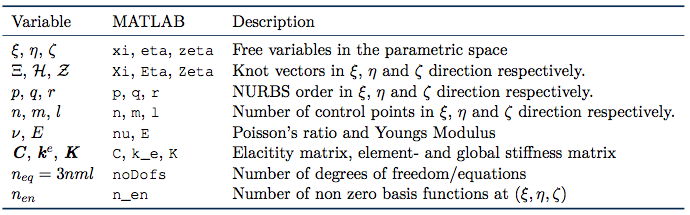
Initially the IGA implementation was entirely based on the library given in the article “Isogeometric analysis: an overview and computer implementation aspects”. This library have implemented NURBS calculations in C, and have a lot of other artillery which we will not need. We have rewritten all code implemented in C into MATLAB, and many more adjustments have been done, even some optimalizations concerning how the sparse global stiffness matrix is built. In this regard it must be noted that the original code written in C is faster then the corresponding rewritten code in MATLAB. It was not necessary to rewrite all parts of the library, so only the parts which are edited will be presented in whats follows. For the remaining part of the code, we refer to the article “Isogeometric analysis: an overview and computer implementation aspects”. When presenting the theory, we shall consecutively present the corresponding implementation in MATLAB. In this regard we present explanations for the most important variables used, and writes the corresponding variable names used in MATLAB, in the table below.

Screen Shot 2014-05-03 at 18.04.13

NURBS

The NURBS basis is built by B-splines. So an understanding of B-splines is crucial to understanding NURBS. Let $p$ be the polynomial order, let $n$ be the number of functions and let $\Xi = \{\xi_1,\xi_2,\dots,\xi_{n+p+1}\}$ be an ordered vector with non decreasing elements (referred to as a knot vector). Then, the B-spline $N_{i,p}$ are recursively defined by (for $p=0$ )

(1) $\begin{equation*} N_{i,0}(\xi)=\begin{cases} 1 & \text{if } \xi_i\leq \xi < \xi_{i+1}\\ 0 & \text{otherwise} \end{cases} \end{equation*}$

and for $p=1,2,3,\dots$ we have

$\begin{equation*} N_{i,p}(\xi) = \frac{\xi-\xi_i}{\xi_{i+p}-\xi_i}N_{i,p-1}(\xi)+\frac{\xi_{i+p+1} - \xi}{\xi_{i+p+1} -\xi_{i+1}}N_{i+1,p-1}(\xi). \end{equation*}$

This forumla is referred to as Cox-deBoor formula, and the derivative of a spline may be computed by

$\begin{equation*} \frac{d}{d\xi} N_{i,p}(\xi) = \frac{p}{\xi_{i+p}-\xi_{i}}N_{i,p-1}(\xi)-\frac{p}{\xi_{i+p+1}-\xi_{i+1}}N_{i+1,p-1}(\xi). \end{equation*}$

Throughout the project we shall use open knot vectors. That is, the first and last element in the vector is repeated $p+1$ times. Moreover, we shall use normalized knot vectors, which simply spans from 0 to 1. We shall build upon this information to optimize algorithms. When we want to evaluate a B-spline at a fixed $\xi$ it is important to note that it is very redundant to evaluate all $n$ basis function. This is due to the small support of each function. In fact, it turns out that only (at most) $p+1$ basis functions are non-zero at $\xi$ . It is important to then only use these function to have an efficient code. One typically then implements a function which find the span corresponding to a given $\xi$ . Due to the ordering of the knot vector, we may use a binary search algorithm for finding this span. 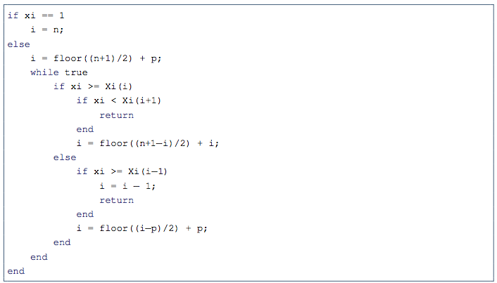The span will be defined by the index $i$ corresponding to the first basis function which is non-zero at $\xi$ . The following listing represents the algorithm called findKnotSpan.m:

Screen Shot 2014-05-03 at 18.15.54

As an example, if $p=2$ and $n=8$ and we want to evaluate a B-spline with the knot vector $\Xi = \{0, 0, 0, 0.1, 0.3, 0.5, 0.8, 0.9, 1, 1, 1\}$ , we get the index $i=3$ if $\xi = 0.09$ , $i=6$ if $\xi=0.5$ and $i=n=8$ if $\xi=0.9$ or $\xi = 1.0$ .

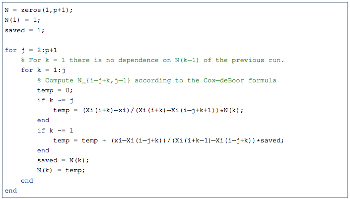
We are now ready to implmenet a program which evaluates B-splines using the previous routine. When the recursion formula is used to evaluate the $p+1$ functions which are non-zero at $\xi$ , the function $N_{i,0}$ is the only function of order zero which is non-zero at $\xi$ . Everything is thus build from this function. We then have the following graph

Screen Shot 2014-05-03 at 18.18.29

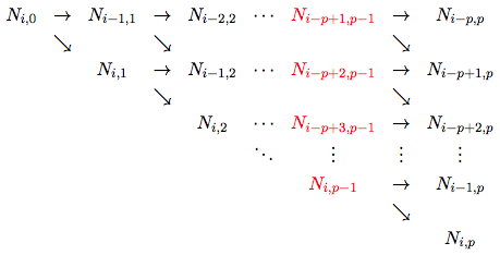
where the values colored red is used to calculate the nonzero derivatives at the same $\xi$ . It is then clear that we need two loops. The outer loop should iterate over the columns of this graph and the inner loop should iterate over the rows. The output of the function Bspline_basis is simply an array N which contains the $p+1$ functions which are evaluated at $\xi$ . To save memory one should also store the intermediate values $N_{i-j+k, j-1}$ in this same array. Thus, we need to store N(k-1) to compute N(k) (which we store in the variable saved). Here, $j$ is the loop index of the outer loop, while $k$ is the loop index of the inner loop. The first iteration (when $p=0$ ) should be done seperately with 1. Finally, we use the convention that $0/0 = 0$ .

Screen Shot 2014-05-03 at 18.16.08

A way to veryfy this implementation is to check that the nonegativity and the partion of unity holds,

$\begin{equation*} N_{i,p}(\xi)\geq 0 \quad\text{and}\quad\sum_{i=1}^n N_{i,p}(\xi) = 1\qquad\forall \xi, p, \end{equation*}$

which is important properties of B-splines. We will finally need to compute the corresponding derivatives. Once again, only $p+1$ derivatives will be non zero at $\xi$ . Let N_tilde be an array containing the red values in the previous graph. We may then compute these as in the following listing

Screen Shot 2014-05-03 at 18.16.13

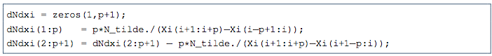
Since we only need these derivatives also when the corresponding values for the basis function is needed, we extend the function Bspline_basis into a new function called Bspline_basisDers. We then avoid redundant calculations.

A B-spline volume may now be represented by

(2) $\begin{equation*} \vec{V}(\xi,\eta,\zeta) = \sum_{i=1}^n\sum_{j=1}^m\sum_{k=1}^l N_{i,p}(\xi)M_{j,q}(\eta)L_{k,r}(\zeta)\vec{P}_{i,j,k} \end{equation*}$

where $\vec{P}$ contains the $n\cdot m\cdot l$ controlpoint of the volume. For a given $(\xi,\eta,\zeta)$ , this formula does a lot of redundant computations as discussed so far. Namely, given a $(\xi,\eta,\zeta)$ , only $(p+1)\cdot(q+1)\cdot(r+1)$ basis functions will contribute. If these nonzero basis functions evaluated at a given point $(\xi,\eta,\zeta)$ are stored in M, N and L, we may rewrite 2 as

$\begin{equation*} \vec{V}(\xi,\eta,\zeta) = \sum_{k_1=1}^{p+1}\sum_{k_2=1}^{q+1}\sum_{k_3=1}^{r+1} \underbrace{N_{A_1,p}(\xi)}_{N(k1)}\underbrace{M_{A_2,q}(\eta)}_{M(k2)}\underbrace{L_{A_3,r}(\zeta)}_{L(k3)}\vec{P}_{A_1,A_2,A_3} \end{equation*}$

where

$\begin{align*} A_1 &= i_1-p+k_1-1\\ A_2 &= i_2-q+k_2-1\\ A_3 &= i_3-r+k_3-1 \end{align*}$

and $i_1$ , $i_2$ and $i_3$ are knot span index corresponding to $\xi$ , $\eta$ and $\zeta$ , respectively. This observation will be used frequently when dealing with corresponding sums in the NURBS basis.

Given a set of weights $w$ corresponding to each basis function the NURBS basis functions in 3D may be expressed by

(3) $\begin{equation*} R_{i,j,k}^{p,q,r}(\xi,\eta,\zeta) = \frac{N_{i,p}(\xi)M_{j,q}(\eta)L_{k,r}(\zeta)w_{i,j,k}}{W(\xi,\eta,\zeta)} \end{equation*}$

where

$\begin{equation*} W(\xi,\eta,\zeta) = \sum_{k_1=1}^{p+1}\sum_{k_2=1}^{q+1}\sum_{k_3=1}^{r+1} \underbrace{N_{A_1,p}(\xi)}_{N(k1)}\underbrace{M_{A_2,q}(\eta)}_{M(k2)}\underbrace{L_{A_3,r}(\zeta)}_{L(k3)}w_{A_1,A_2,A_3}. \end{equation*}$

The partial derivatives of these functions is then given by the quotient rule

(4) $\begin{equation*} \frac{\partial R_{i,j,k}^{p,q,r}(\xi,\eta,\zeta)}{\partial \xi} = \frac{W(\xi,\eta,\zeta)N_{i,p}'(\xi) - W_\xi(\xi,\eta,\zeta)N_{i,p}(\xi)}{(W(\xi,\eta,\zeta))^2}M_{j,q}(\eta)L_{k,r}(\zeta)w_{i,j,k} \end{equation*}$

where

$\begin{equation*} W_\xi(\xi,\eta,\zeta) = \sum_{k_1=1}^{p+1}\sum_{k_2=1}^{q+1}\sum_{k_3=1}^{r+1} \underbrace{N_{A_1,p}'(\xi)}_{dNdxi(k1)}\underbrace{M_{A_2,q}(\eta)}_{M(k2)}\underbrace{L_{A_3,r}(\zeta)}_{L(k3)}w_{A_1,A_2,A_3} \end{equation*}$

and

$\begin{equation*} N_{i,p}'(\xi) = \frac{d N_{i,p}(\xi)}{d\xi}. \end{equation*}$

Similar expressions may be found for the partial derivatives with respect to $\eta$ and $\zeta$ . We may now insert all of this into a routine which computes the nonzero basis functions at a given point $(\xi,\eta,\zeta)$ and the corresponding nonzero derivatives. This function is called NURBS3DBasisDers. After finding the nonzero B-spline functions and their corresponding derivatives as discussed above, it continues by first finding the function $W$ and it’s corresponding derivatives. This is illustrated in the following listing.

Screen Shot 2014-05-03 at 18.16.47

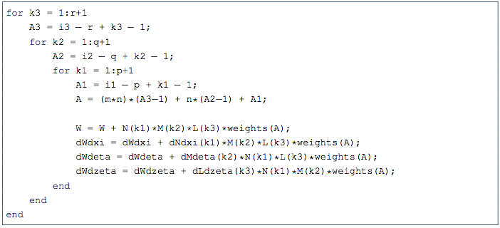
Note the use of the index A which is convenient when weights is located in an long array (which is the format we shall use when doing the IGA analysis). Finally, the function can now compute the NURBS basis alongside the corresponding derivatives as shown in the following listing.

Screen Shot 2014-05-03 at 18.16.59

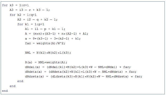
Note the use of the intermediate variables fac and NML which is used to avoid redundant computations. The index a loops over the $n_{en}=(p+1)\cdot(q+1)\cdot(r+1)$ nonzero functions.

Linear elasticity

One important assumption for using linear elasticity is that only small deformations of the material occurs. This is due to the linearized quantities. We shall here not go in detail on how to derive the needed equations from Hooke’s law, but we present the notation used in the formulation of the isogeometric analysis.

The notations used, takes inspirations from the book by Hughes. In this section, the indices $i$ , $j$ , $k$ and $l$ will denote a specific spatial direction. We shall model everything in three dimensions, such that $i,j,k,l=1,2,3$ . Moreover, $u_i$ shall denote the $i^{\textnormal{th}}$ component of the vector $\vec{u}$ and differentiation is denoted with a comma such that

$\begin{equation*} u_{i,j} = u_{i,x_j} =\frac{\partial u_i}{\partial x_j}. \end{equation*}$

Finally, we use the convention that if an index is repeated, it imply summation. That is,

$\begin{equation*} \sigma_{ij} n_j = \sigma_{i,1} n_1 + \sigma_{i,2} n_2 + \sigma_{i,3} n_3 \end{equation*}$

and

$\begin{equation*} \sigma_{ij,j} + f_i = \frac{\partial\sigma_{i1}}{\partial x_1} + \frac{\partial\sigma_{i2}}{\partial x_2} + \frac{\partial\sigma_{i3}}{\partial x_3} + f_i. \end{equation*}$

Note that we do not sum over $i$ in the latter example since the quantities are separated by a plus sign. Define now the symmetric part of a general tensor $\vec{A}=[A_{ij}]$ to be

$\begin{equation*} A_{(ij)} = A_{(ji)} := \frac{A_{ij}+A_{ji}}{2} \end{equation*}$

and note that if $\vec{B}=[B_{ij}] = [B_{(ij)}]$ is a symmetric tensor, then

(5) $\begin{equation*} A_{ij} B_{ij} = A_{(ij)} B_{ij}. \end{equation*}$

That is, we can combine the components of $\vec{B}$ which are equal to reduce redundant computations.

Let now $\sigma_{ij}$ denote the Cartesian components of the Cauchy stress tensor and let $\varepsilon_{ij}$ denote the infinitesimal strain tensor which is defined by

$\begin{equation*} \varepsilon_{ij} = u_{(i,j)} = \frac{u_{i,j}+u_{j,i}}{2}. \end{equation*}$

We can now state the relation between $\varepsilon_{ij}$ as $\sigma_{ij}$ using the generalized Hooke’s law as

$\begin{equation*} \sigma_{ij} = c_{ijkl}\varepsilon_{kl} \end{equation*}$

where $c_{ijkl}$ are elastic coefficients. In the case of isotropic material, these coefficients are given by

$\begin{equation*} c_{ijkl} = \frac{\nu E}{(1+\nu)(1-2\nu)}\delta_{ij}\delta_{kl} + \frac{E}{2(1+\nu)}\left(\delta_{ik}\delta_{jl}+\delta_{il}\delta_{jk}\right) \end{equation*}$

where the Kronecker delta function is given by

$\begin{equation*} \delta_{ij}=\begin{cases} 1 &i=j\\ 0&\text{otherwise} \end{cases} \end{equation*}$

and the parameters $E$ and $\nu$ are Young’s modulus and Poisson’s ratio respectively. We are now ready to state the strong form of the linear elasticity problem in three dimensions.

Let $\Omega\subset\mathbb{R}^3$ be the domain with a boundary $\partial \Omega$ which is composed of two parts; $\Gamma_{D_i}$ and $\Gamma_{N_i}$ . These are called Dirichlet and Neumann boundary conditions, respectively, and satisfies $\bigcup_{i=1}^3\Gamma_{D_i}\cup\Gamma_{N_i}=\partial\Omega$ and $\Gamma_{D_i}\cap\Gamma_{N_i}=\emptyset$ . Moreover, let the functions $f_i:\Omega\to\mathbb{R}$ , $g_i:\Gamma_{D_i}\to\mathbb{R}$ and $h_i:\Gamma_{N_i}\to\mathbb{R}$ be given. Then, find $u_i:\overline{\Omega}\to\mathbb{R}$ such that

(6) $\begin{alignat*}{3} \sigma_{ij,j} + f_i &= 0\qquad &&\text{in}\quad \Omega,\\ u_i &= g_i &&\text{on}\quad \Gamma_{D_i},\\ \sigma_{ij} n_j &= h_i &&\text{on}\quad \Gamma_{N_i}, \end{alignat*}$

for $i=1,2,3$ . In this project, we will only consider boundaries which are entirely Neumann boundaries or Dirichlet boundaries, respectively. That is, $\Gamma_{D_i} = \Gamma_D$ and $\Gamma_{N_i} = \Gamma_{N}$ for all $i$ .

In this project, we neglect any body forces such as gravity, such that $f_i=0$ . Moreover, we shall only need homogeneous Dirichlet conditions such that $g_i=0$ .

The weak form and Galerkin’s Method

The weak form of the problem is derived from the strong form. Typically, one defines two classes of functions: $\mathcal{S}_i$ denotes the solution space and $\mathcal{V}_i$ denotes the weighting space for a given spatial component $i$ . These spaces are made in order to handle non homogeneous Dirichlet boundary conditions, but since we have homogeneous Dirichlet boundary conditions, these spaces will be the same. That is, $\mathcal{S}_i=\mathcal{V}_i$ for $i=1,2,3$ . Typically, $\mathcal{S}_i$ is a subspace of the Sobolev space $H^1(\Omega)$ (which consist of all functions which have square-integrable derivatives) with a condition such that the Dirichlet boundary condition is satisfied.

We now multiply each of the equations in 6 by a corresponding test functions $v_i\in\mathcal{S}_i$ and sum these three equations into one single equation given by

$\begin{equation*} v_i\sigma_{ij,j} = -v_i f_i \end{equation*}$

which can be written as

$\begin{equation*} v_i\nabla\cdot\bar{\boldsymbol\sigma}_i = -v_i f_i \end{equation*}$

where

$\begin{equation*} \bar{\boldsymbol\sigma}_i = \begin{bmatrix} \sigma_{i1}\\ \sigma_{i2}\\ \sigma_{i3} \end{bmatrix}. \end{equation*}$

Integrating over the domain yields

(7) $\begin{equation*} \int_\Omega v_i\nabla\cdot\bar{\boldsymbol\sigma}_i\idiff\Omega = -\int_\Omega v_i f_i\idiff\Omega. \end{equation*}$

Consider the divergence theorem

$\begin{equation*} \int_\Omega\nabla\cdot \boldsymbol\Psi\idiff\Omega = \int_{\partial\Omega} \boldsymbol\Psi\cdot \vec{n}\idiff\Omega \end{equation*}$

with $\boldsymbol\Psi=v_i\bar{\boldsymbol\sigma}_i$ . Note that

$\begin{equation*} \nabla\cdot \boldsymbol\Psi = \nabla\cdot(v_i\bar{\boldsymbol\sigma}_i) = \nabla v_i\cdot\bar{\boldsymbol\sigma}_i + v_i\nabla\cdot\bar{\boldsymbol\sigma}_i \end{equation*}$

which inserted in the divergence theorem yields

$\begin{equation*} \int_\Omega v_i\nabla\cdot\bar{\boldsymbol\sigma}_i\idiff\Omega = -\int_\Omega\nabla v_i\cdot\bar{\boldsymbol\sigma}_i\idiff\Omega + \int_{\partial\Omega} v_i\bar{\boldsymbol\sigma}_i\cdot \vec{n}\idiff\Omega. \end{equation*}$

We may now insert this into 7 such that

(8) $\begin{equation*} \int_\Omega\nabla v_i\cdot\bar{\boldsymbol\sigma}_i\idiff\Omega = \int_{\Gamma_N} v_i\bar{\boldsymbol\sigma}_i\cdot \vec{n}\idiff\Omega + \int_\Omega v_i f_i\idiff\Omega. \end{equation*}$

Note that we only integrate over the Neumann part of the boundary since the integral over the vanishes (the test function $v_i$ is zero at this boundary). Also note that the domain of integration for the boundary integral is depending on $i$ . Returning to the index summation convention we may rewrite 8 as

$\begin{equation*} \int_\Omega v_{i,j}\sigma_{ij}\idiff\Omega = \int_{\Gamma_N} v_i(\sigma_{ij} n_j)\idiff\Gamma + \int_\Omega v_i f_i\idiff\Omega \end{equation*}$

which using the boundary conditions, and the fact that $f_i=0$ for our case, may be written as

$\begin{equation*} \int_\Omega v_{(i,j)}\sigma_{ij}\idiff\Omega = \int_{\Gamma_N} v_i h_j\idiff\Gamma. \end{equation*}$

Note that since $[\sigma_{ij}]$ is a symmetric tensor, we have used 5 to only write the symmetric part of $v_{i,j}$ . If we now define the space $\boldsymbol{\mathcal{S}}=\{\vec{u}\,|\,u_i\in\mathcal{S}_i\}$ we can state the weak formulation in a concise form: Find $\vec{u}\in\boldsymbol{\mathcal{S}}$ such that for all $\vec{v}\in\boldsymbol{\mathcal{S}}$ we have

$\begin{equation*} a(\vec{v},\vec{u}) = L(\vec{v}) \end{equation*}$

where

(9) $\begin{equation*} a(\vec{v},\vec{u}) = \int_\Omega v_{(i,j)}c_{ijkl}u_{(k,l)}\idiff\Omega \end{equation*}$

and

$\begin{equation*} L(\vec{v}) = \int_{\Gamma_N} v_i h_j\idiff\Gamma. \end{equation*}$

Here we have used the relation $\sigma_{ij} = c_{ijkl}\varepsilon_{kl} = c_{ijkl}u_{(k,l)}$ .

We now want to transform this weak statement into a system of algebraic equations. We here apply Galerkin’s method and now turn to a finite-dimensional subspace $\boldsymbol{\mathcal{S}}^h\subset \boldsymbol{\mathcal{S}}$ . The basis for this subspace is the presented NURBS basis. But note that we will have vector valued control variables. The Galerkin approximation of the weak form is now given by: Find $\vec{u}^h\in\boldsymbol{\mathcal{S}}^h$ such that

(10) $\begin{equation*} a(\vec{v}^h,\vec{u}^h) = L(\vec{v}^h) \end{equation*}$

for all $\vec{v}^h\in\boldsymbol{\mathcal{S}}^h$ .

To find the system of algebraic equations we need to write $\vec{u}^h$ as a linear combination of the basis functions. First, let $\boldsymbol\eta=\{1,\dots,n_{np}\}$ (where $n_{np}$ is the number of basis functions) be the set containing the indices of all the functions in the NURBS basis defining the geometry and let $\boldsymbol\eta_{g_i}\subset \boldsymbol\eta$ be the set containing the indices of all the basis functions that are non-zero on $\Gamma_D$ . Due to the homogeneous Dirichlet boundary condition, we may write the $i^{\textnormal{th}}$ component of $\vec{v}^h$ and the $j^{\textnormal{th}}$ component of $\vec{u}^h$ as

(11) $\begin{equation*} v_i^h = \sum_{A\in\boldsymbol\eta-\boldsymbol\eta_{g_i}} R_A c_{iA}\quad\text{and}\quad u_j^h = \sum_{B\in\boldsymbol\eta-\boldsymbol\eta_{g_j}} R_A d_{jB} \end{equation*}$

respectively, where $\boldsymbol\eta-\boldsymbol\eta_{g_i}$ denotes set subtraction. Using the same index summation convention we may now write

(12) $\begin{equation*} \vec{v}^h = v_i^h \vec{e}_i\quad\text{and}\quad \vec{u}^h = u_j^h \vec{e}_j \end{equation*}$

where the unit vectors $\vec{e}_i$ are given by

$\begin{equation*} \vec{e}_1=\begin{bmatrix} 1\\ 0\\ 0 \end{bmatrix},\quad\vec{e}_2=\begin{bmatrix} 0\\ 1\\ 0 \end{bmatrix},\quad\text{and}\quad\vec{e}_3=\begin{bmatrix} 0\\ 0\\ 1 \end{bmatrix}. \end{equation*}$

The finale step is now to insert 12 (using 11) into 10 such that we obtain a matrix formulation of the problem. Insertion yields

$\begin{equation*} a\left(\sum_{A\in\boldsymbol\eta-\boldsymbol\eta_{g_j}} R_A c_{iA}\vec{e}_i, \sum_{B\in\boldsymbol\eta-\boldsymbol\eta_{g_i}} R_B d_{jB}\vec{e}_j\right) - L\left(\sum_{A\in\boldsymbol\eta-\boldsymbol\eta_{g_i}} R_A c_{iA}\vec{e}_i\right) = 0 \end{equation*}$

which using the bilinearity of $a$ and the linearity of $L$ may be written as

$\begin{equation*} \sum_{A\in\boldsymbol\eta-\boldsymbol\eta_{g_i}}c_{iA}\left(\sum_{B\in\boldsymbol\eta-\boldsymbol\eta_{g_i}} a\left(R_A\vec{e}_i, R_B \vec{e}_j\right)d_{jB} - L\left(R_A\vec{e}_i\right)\right) = 0. \end{equation*}$

Since the coefficients $c_{iA}$ is arbitrary (the relation should hold for all $\vec{v}^h\in \boldsymbol{\mathcal{S}}^h$ ) the term in the parentheses must vanish. That is, for all $A\in\boldsymbol\eta-\boldsymbol\eta_{g_i}$ and $i=1,2,3$ we have

$\begin{equation*} \sum_{B\in\boldsymbol\eta-\boldsymbol\eta_{g_i}} a\left(R_A\vec{e}_i, R_B \vec{e}_j\right)d_{jB} = L\left(R_A\vec{e}_i\right). \end{equation*}$

One should typically make a system of the ordering of these equations. That is, one should create a function $\mathrm{ID}$ which collapse the indices $i$ and $A$ into a single index. A given equation then has the index $P=\mathrm{ID}(i,A)$ and the index over all unknown components of the displacement vectors are called $Q=\mathrm{ID}(j,B)$ . The resulting system of equation may then be written as

$\begin{equation*} \vec{K} \vec{U}=\vec{F} \end{equation*}$

where

$\begin{equation*} \vec{K} = [K_{PQ}],\\ \vec{U} = \{d_Q\},\\ \vec{F} = \{F_P\}, \end{equation*}$

and

$\begin{equation*} K_{PQ}=a\left(R_A\vec{e}_i,R_B\vec{e}_j\right),\\ F_P=L(R_A\vec{e}_j),\\ d_Q=d_{jB}. \end{equation*}$

Assembly

As for the finite element method, one typically do not loop through the basis functions. Rather, we loop through the elements constructing local stiffness matrices and successfully place their element in the global stiffness matrix. Let us first introduce some notations. The elastic coefficients are typically inserted in a matrix $\vec{C}$ called the elasticity matrix. It is defined by

$\begin{equation*} \vec{C} = \begin{bmatrix} c_{1111} & c_{1122} & c_{1133} & c_{1123} & c_{1113} & c_{1112}\\ & c_{2222} & c_{2233} & c_{2223} & c_{2213} & c_{2212}\\ & & c_{3333} & c_{3323} & c_{3313} & c_{3312}\\ & & & c_{2323} & c_{2323} & c_{2312}\\ & \multicolumn{2}{c}{\text{symmetric}} & & c_{1313} & c_{1312}\\ & & & & & c_{1212} \end{bmatrix}, \end{equation*}$

or in our case, more explicitly by

$\begin{equation*} \vec{C} = \frac{E}{(1+\nu)(1-2\nu)}\begin{bmatrix} 1-\nu & \nu & \nu & 0 & 0 & 0\\ \nu & 1-\nu & \nu & 0 & 0 & 0\\ \nu & \nu & 1-\nu & 0 & 0 & 0\\ 0 & 0 & 0 & (1-2\nu)/2 & 0 & 0\\ 0 & 0 & 0 & 0 & (1-2\nu)/2 & 0\\ 0 & 0 & 0 & 0 & 0 & (1-2\nu)/2 \end{bmatrix}. \end{equation*}$

Moreover, define the strain vector and the stress vector to be

$\begin{equation*} \boldsymbol\varepsilon(\vec{u}) = \begin{bmatrix} u_{1,1}\\ u_{2,2}\\ u_{3,3}\\ u_{2,3} + u_{3,2}\\ u_{3,1} + u_{1,3}\\ u_{1,2} + u_{2,1} \end{bmatrix}\quad\text{and}\quad \boldsymbol\sigma = \begin{bmatrix} \sigma_{11}\\ \sigma_{22}\\ \sigma_{33}\\ \sigma_{23}\\ \sigma_{13}\\ \sigma_{12}\\ \end{bmatrix}. \end{equation*}$

Then

$\begin{equation*} \boldsymbol\sigma = \vec{C}\boldsymbol\varepsilon(\vec{u}), \end{equation*}$

such that we may write the bilinear form in 9 as

$\begin{equation*} a(\vec{v},\vec{u}) = \int_\Omega \boldsymbol\varepsilon(\vec{v})^\transpose \vec{C}\boldsymbol\varepsilon(\vec{u}) \idiff\Omega. \end{equation*}$

Also note that

$\begin{equation*} \boldsymbol\varepsilon(R_A\vec{e}_i) = \vec{B}_A\vec{e}_i, \end{equation*}$

where

$\begin{equation*} \vec{B}_A = \begin{bmatrix} R_{A,1} & 0 & 0\\ 0 & R_{A,2} & 0\\ 0 & 0 & R_{A,3}\\ 0 & R_{A,3} & R_{A,2}\\ R_{A,3} & 0 & R_{A,1}\\ R_{A,2} & R_{A,1} & 0 \end{bmatrix}. \end{equation*}$

The entries in the global stiffness matrix may then be written as

$\begin{equation*} K_{PQ}=a\left(R_A\vec{e}_i,R_B\vec{e}_j\right) = \vec{e}_i^\transpose\int_\Omega \vec{B}_A^\transpose \vec{C}\vec{B}_B \idiff\Omega\, \vec{e}_j. \end{equation*}$

Let $\Omega^e$ be the domain of a given element, where the index $e$ loops over all elements. The support of the NURBS are highly localized. To reduce computations, we should only integrate over functions which have support in $\Omega^e$ . If we have $n_{en}$ such \local shape functions, and let $a$ and $b$ iterate over these functions, we may calculate the entries in the local stiffness matrix as

$\begin{equation*} k_{pq}^e = \vec{e}_i^\transpose\int_{\Omega^e} \vec{B}_a^\transpose \vec{C}\vec{B}_b \idiff\Omega\, \vec{e}_j \end{equation*}$

where

$\begin{equation*} p = n_{en}(i-1)+a\quad\text{and}\quad q=n_{en}(j-1)+b. \end{equation*}$

The local force vector may similarly be calculated by

(13) $\begin{equation*} f_p^e = \int_{\Gamma_N^e} R_A h_i\idiff\Gamma. \end{equation*}$

The integration is done by quadrature formulas. One first maps to the parametric domain, and then map this domain to a parent domain. The element in the parametric domain, corresponding to $\Omega^e$ , is given by

$\begin{equation*} \hat{\Omega}^e= [\xi_i,\xi_{i+1}]\times[\eta_i,\eta_{i+1}]\times[\zeta_i,\zeta_{i+1}]. \end{equation*}$

In three dimension we want to map this domain into the parent domain given by

$\begin{equation*} \tilde{\Omega}^e = [-1,1]\times[-1,1]\times[-1,1]. \end{equation*}$

So given $(\tilde{\xi},\tilde{\eta},\tilde{\zeta})\in \tilde{\Omega}^e$ , we calculate $(\xi,\eta,\zeta)\in \hat{\Omega}^e$ by

$\begin{equation*} \xi = \xi_i + (\tilde{\xi}+1)\frac{\xi_{i+1}-\xi_i}{2}, \end{equation*}$

$\begin{equation*} \eta = \eta_i + (\tilde{\eta}+1)\frac{\eta_{i+1}-\eta_i}{2}, \end{equation*}$

$\begin{equation*} \zeta = \zeta_i + (\tilde{\zeta}+1)\frac{\zeta_{i+1}-\zeta_i}{2}. \end{equation*}$

The Jacobian determinant for the parametric to parent mapping is thus given by

$\begin{equation*} J_2 = \begin{vmatrix} \frac{\partial \xi}{\partial\tilde{\xi}} & \frac{\partial \xi}{\partial\tilde{\eta}} & \frac{\partial \xi}{\partial\tilde{\zeta}}\\ \frac{\partial \eta}{\partial\tilde{\xi}} & \frac{\partial \eta}{\partial\tilde{\eta}} & \frac{\partial \eta}{\partial\tilde{\zeta}}\\ \frac{\partial \zeta}{\partial\tilde{\xi}} & \frac{\partial \zeta}{\partial\tilde{\eta}} & \frac{\partial \zeta}{\partial\tilde{\zeta}}\\ \end{vmatrix}=\frac{1}{8}(\xi_{i+1}-\xi_i)(\eta_{i+1}-\eta_i)(\zeta_{i+1}-\zeta_i). \end{equation*}$

Similarly, we need the Jacobian for the mapping from the physical domain into the parametric domain. Given $(\xi,\eta,\zeta)\in \hat{\Omega}^e$ , we calculate $(x,y,z) = (x_1,x_2,x_3)\in \Omega^e$ by

$\begin{equation*} \begin{bmatrix} x_1\\ x_2\\ x_3 \end{bmatrix} = \sum_{i=1}^n\sum_{j=1}^m\sum_{k=1}^l R_{i,j,k}^{p,q,r}(\xi,\eta,\zeta) \vec{P}_{i,j,k} = \sum_{a=1}^{n_{en}} R_a(\xi,\eta,\zeta) \vec{P}_a \end{equation*}$

where $\vec{P}_{i,j,k}$ are the control points and $R_{i,j,k}^{p,q,r}(\xi,\eta,\zeta)$ are the NURBS basis functions which are computed by 3. Note that the last equality again comes from the highly localized support of the NURBS basis. The Jacobian matrix is thus given by

$\begin{equation*} \vec{J} = \begin{bmatrix} \frac{\partial x_1}{\partial \xi} & \frac{\partial x_1}{\partial \eta} & \frac{\partial x_1}{\partial \zeta}\\ \frac{\partial x_2}{\partial \xi} & \frac{\partial x_2}{\partial \eta} & \frac{\partial x_2}{\partial \zeta}\\ \frac{\partial x_3}{\partial \xi} & \frac{\partial x_3}{\partial \eta} & \frac{\partial x_3}{\partial \zeta} \end{bmatrix} = \begin{bmatrix} \vec{P}_1 & \vec{P}_2 & \cdots & \vec{P}_{n_{en}} \end{bmatrix}\begin{bmatrix} \frac{\partial R_1}{\partial \xi} & \frac{\partial R_1}{\partial \eta} & \frac{\partial R_1}{\partial \zeta}\\ \frac{\partial R_2}{\partial \xi} & \frac{\partial R_2}{\partial \eta} & \frac{\partial R_2}{\partial \zeta}\\ \vdots &\vdots &\vdots \\ \frac{\partial R_{n_{en}}}{\partial \xi} & \frac{\partial R_{n_{en}}}{\partial \eta} & \frac{\partial R_{n_{en}}}{\partial \zeta}\\ \end{bmatrix} \end{equation*}$

such that the Jacobian determinant of this transformation is given by

$\begin{equation*} J_1 = \mathrm{det}(\vec{J}) \end{equation*}$

where the derivatives of the NURBS basis functions are computed by 4. The matrix $\vec{B}_a$ contains derivatives of the NURBS functions w.r.t. physical coordinates. So we need to find expressions for $\frac{\partial R}{\partial x_i}$ . By the chain rule we have

$\begin{equation*} \frac{\partial R}{\partial \xi} = \frac{\partial R}{\partial x_1}\frac{\partial x_1}{\partial \xi} + \frac{\partial R}{\partial x_2}\frac{\partial x_2}{\partial \xi} + \frac{\partial R}{\partial x_3}\frac{\partial x_3}{\partial \xi} \end{equation*}$

$\begin{equation*} \frac{\partial R}{\partial \eta} = \frac{\partial R}{\partial x_1}\frac{\partial x_1}{\partial \eta} + \frac{\partial R}{\partial x_2}\frac{\partial x_2}{\partial \eta} + \frac{\partial R}{\partial x_3}\frac{\partial x_3}{\partial \eta} \end{equation*}$

$\begin{equation*} \frac{\partial R}{\partial \zeta} = \frac{\partial R}{\partial x_1}\frac{\partial x_1}{\partial \zeta} + \frac{\partial R}{\partial x_2}\frac{\partial x_2}{\partial \zeta} + \frac{\partial R}{\partial x_3}\frac{\partial x_3}{\partial \zeta}. \end{equation*}$

And thus, we may write

(14) $\begin{equation*} \begin{bmatrix} \frac{\partial R}{\partial x_1} & \frac{\partial R}{\partial x_2}& \frac{\partial R}{\partial x_3} \end{bmatrix}\vec{J} = \begin{bmatrix} \frac{\partial R}{\partial \xi} & \frac{\partial R}{\partial \eta}& \frac{\partial R}{\partial \zeta} \end{bmatrix}. \end{equation*}$

Multiplying with the inverse of the Jacobian, $\vec{J}^{-1}$ , from the right and taking the transpose on each side of the equation finally yields

$\begin{equation*} \begin{bmatrix} \frac{\partial R}{\partial x_1}\\ \frac{\partial R}{\partial x_2}\\ \frac{\partial R}{\partial x_3} \end{bmatrix} = \vec{J}^{-\transpose} \begin{bmatrix} \frac{\partial R}{\partial \xi}\\ \frac{\partial R}{\partial \eta}\\ \frac{\partial R}{\partial \zeta} \end{bmatrix}. \end{equation*}$

By successfully placing these expressions in the matrix $\vec{B}$ , we may finally write

$\begin{equation*} k_{pq}^e = \vec{e}_i^\transpose\int_{\tilde{\Omega}^e} \vec{B}_a^\transpose \vec{C}\vec{B}_b |J_1||J_2| \idiff\tilde{\Omega}\, \vec{e}_j. \end{equation*}$

By carefully sequentially placing all values for $a,b=1,\dots,n_{en}$ into the matrix $\vec{B}$ we can compute the whole local stiffness matrix in one go by

$\begin{equation*} \vec{k}^e = \int_{\tilde{\Omega}^e} \vec{B}^\transpose \vec{C}\vec{B} |J_1||J_2| \idiff\tilde{\Omega}. \end{equation*}$

The integrals is approximated with quadrature rules. If we want to approximate the integral

$\begin{equation*} \int_{\tilde{\Omega}} g(\tilde{\xi}, \tilde{\eta}, \tilde{\zeta}) \idiff \tilde{\Omega} \end{equation*}$

the approximation by Gaussian quadrature is given by

$\begin{equation*} \int_{\tilde{\Omega}} g(\tilde{\xi}, \tilde{\eta}, \tilde{\zeta}) \idiff \tilde{\Omega} \approx \sum_{q=1}^{n_q} \rho_q g(\tilde{\xi}_q, \tilde{\eta}_q, \tilde{\zeta}_q), \end{equation*}$

where $n_q$ are the number of integration points, and $(\tilde{\xi}_q, \tilde{\eta}_q, \tilde{\zeta}_q)$ and $\rho_q$ are given quadrature points and weights, respectively.

A somewhat similar procedure as shown above is needed to approximate the surface integral in \eqref{Eq:loading}. The full expression will depend on which part of the surface we integrate over. As an example, consider integrating over a surface where $\eta=0$ . As for the local stiffness matrix, we can compute the corresponding contribution to the load vector in one go as follows

$\begin{equation*} \vec{f}^e = \int_{\tilde{\Gamma}_{N}^e} \begin{bmatrix} \vec{R}^\transpose\Big\vert_{\eta=0}h_1 & \vec{R}^\transpose\Big\vert_{\eta=0}h_2 & \vec{R}^\transpose\Big\vert_{\eta=0}h_3\end{bmatrix}^\transpose |J_1||J_2|\idiff\tilde{\Gamma} \end{equation*}$

where

$\begin{equation*} \vec{R}^\transpose = \begin{bmatrix} R_1 & R_2 & \dots & R_{n_{en}} \end{bmatrix}, \end{equation*}$

$\begin{equation*} J_2 = \frac{1}{4}(\xi_{i+1}-\xi_i)(\zeta_{i+1}-\zeta_i), \end{equation*}$

$\begin{equation*} J_1 = \mathrm{det}(\vec{J}), \end{equation*}$

and

$\begin{equation*} \vec{J} = \begin{bmatrix} \frac{\partial x_1}{\partial \xi} & \frac{\partial x_1}{\partial \zeta}\\ \frac{\partial x_3}{\partial \xi} & \frac{\partial x_3}{\partial \zeta} \end{bmatrix} = \begin{bmatrix} \vec{P}'_1 & \vec{P}'_2 & \cdots & \vec{P}'_{n_{en}} \end{bmatrix}\begin{bmatrix} \frac{\partial R_1}{\partial \xi} & \frac{\partial R_1}{\partial \zeta}\\ \frac{\partial R_2}{\partial \xi} & \frac{\partial R_2}{\partial \zeta}\\ \vdots & \vdots\\ \frac{\partial R_{n_{en}}}{\partial \xi} & \frac{\partial R_{n_{en}}}{\partial \zeta}\\ \end{bmatrix}. \end{equation*}$

Here $\vec{P}'_i$ contains the $x_1$ and $x_3$ component of the control point $\vec{P}_i$ . The integral may now be approximated by quadrature rules in two dimensions.

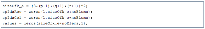
It is very important to note that the global stiffness matrix is very sparse. Not only is it a huge advantage in MATLAB to have the matrix in sparse format when solving the linear system, but also when assembling the matrix. If the matrix is made sparse only after assembly, then the initialization would require MATLAB to allocated place for a full stiffness matrix. This is very memory consuming and should be avoided if one wants to run the program with many degrees of freedom. A matrix in sparse format contains 3 columns; the first two represent the indices in the matrix and the third column represent the corresponding value. A way to do this is to first construct these three columns in three arrays. By noting that each element stiffness matrix has $\left[3(p+1)(q+1)(r+1)\right]^2$ number of components, we initialize the arrays by the following.

Screen Shot 2014-05-03 at 20.17.13

For each element, the element stiffness matrix is then added in the following way.

Screen Shot 2014-05-03 at 20.17.18

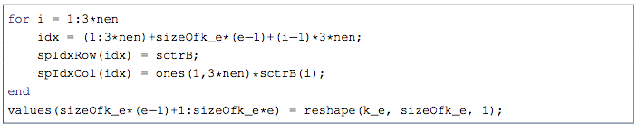
Note that we do not here sum overlapping element matrices, but this is automatically done when the sparse function is called in MATLAB.

That is, there will be index combinations which will repeat and therefore this method would require a lot more memory. The other obvious method is simply using

which typically results in the MATLAB warning “This sparse indexing expression is likely to be slow”. Experimentally we observe that the other method is 5 times as fast.

Post-processing

The visualizations is done in Paraview. Typically we create so called .vts files directly from MATLAB, and let Paraview do the illustrations from here.

We print the nodes, the displacement and every component of the stress for each node into such files. In addition we callculate the von Mises stress given by

$\begin{equation*} \sigma_v = \sqrt{\frac{(\sigma_{11} - \sigma_{22})^2 + (\sigma_{22} - \sigma_{33})^2 + (\sigma_{11} - \sigma_{33})^2 + 6(\sigma_{23}^2 + \sigma_{13}^2 + \sigma_{12}^2)}{2}} \end{equation*}$

which we shall use throughout the report in the visualizations.

One must make a grid in the classical FEM style in order to visualize the result. The mesh is simply created by finding the physical coordinates for each physical element. Moreover, for each corner of an element in the parametric space, the displacement and the components of stress can be calculated. Using the guide in “File formats for vtk version 4.2”, the file writing then follows by looping through each element and write data from each of the 8 corners each time.

MATLAB file structure

Hover the boxes to see subroutines and functions used. Click on a box to be directed to the source file.

Error analysis

It is always important to present some numerical evidence that the implementation is correct. This is typically done by finding an analytic solution and analyze the convergence of the numerical solution towards this analytic solution. Let the minimal order of the NURBS basis be given by

$\begin{equation*} k = \min\{p,q,r\} \end{equation*}$

and let the maximal diameter of the elements (in the parametric space) be noted by $h=h_{max}$ . In the error analysis we shall start by the simplest open knot vectors. That is, for $p=2$ we have $\Xi = \{0, 0, 0, 1, 1, 1\}$ , such that $|\Xi| = n+p+1$ . In three dimensions we then have $h=\sqrt{3}$ . Generally we have

$\begin{equation*} h = \frac{\sqrt{3}}{n-p} \end{equation*}$

where we assume that the polynomial order is equal in all directions and we refine uniformly. The energy norm is defined by

$\begin{equation*} \| \vec{u} - \vec{u}^h\|_E = \sqrt{a(\vec{u} - \vec{u}^h, \vec{u} - \vec{u}^h)} \end{equation*}$

where we compute the bilinear form by

$\begin{equation*} a(\vec{u} - \vec{u}^h,\vec{u} - \vec{u}^h) = \int_\Omega \boldsymbol\varepsilon(\vec{u} - \vec{u}^h)^\transpose \vec{C}\boldsymbol\varepsilon(\vec{u} - \vec{u}^h) \idiff\Omega \end{equation*}$

$\begin{equation*} = \int_\Omega \left[\boldsymbol\varepsilon(\vec{u}) - \boldsymbol\varepsilon(\vec{u}^h)\right]^\transpose \vec{C}\left[\boldsymbol\varepsilon(\vec{u}) - \boldsymbol\varepsilon(\vec{u}^h)\right] \idiff\Omega \end{equation*}$

$\begin{equation*} =\sum_{e=1}^{n_{el}}\int_{\Omega^e}\left[\boldsymbol\varepsilon(\vec{u}) - \boldsymbol\varepsilon(\vec{u}^h)\right]^\transpose \vec{C}\left[\boldsymbol\varepsilon(\vec{u}) - \boldsymbol\varepsilon(\vec{u}^h)\right] \idiff\Omega, \end{equation*}$

using the same technique with transformation to the parent element for integration with quadratures. Thus, we need to compute $\varepsilon(\vec{u})$ in order to do the error analysis.

In the article “Isogeometric analysis using polynomial splines over hierarchical t-meshes for two-dimensional elastic solids” we find the following estimate

$\begin{equation*} \| \vec{u} - \vec{u}^h\|_E \leq C h^{k} \end{equation*}$

where a quasi-uniform mesh refinement has been assumed. The constant $C$ is among other things dependent of the transformation from the parametric space to the physical space. It is not however depending on $h$ . So as $h$ become smaller, we expect the convergence to be of order $k$ . Of course, the analytic solution (and then also the norm) should be independent of $h$ , so we shall divide by $\|\vec{u}\|_E$ to normalize the error.

We want to do an error analysis with an analytic solution and a geometry which is to some extent similar to what we shall use when analyzing the flex of skis. Analytic solution (with corresponding data) on complex domains is in general hard to find. We shall restrict our self to a domain given by

$\begin{equation*} \Omega = (0, w_x)\times (0, w_y)\times (0, w_z) \end{equation*}$

where $w_x$ , $w_y$ and $w_z$ is the width in $x$ , $y$ and $z$ direction of the beam, respectively. In the following we shall present several analytic solutions with corresponding illustrative plots and convergence plots. In the first two cases we choose these three parameters, such that the domain looks like a plank in a way that $w_x>w_y>w_z$ . In all test cases we want to construct solution which have homogeneous Dirichlet boundary conditions at $x=0$ . The boundary conditions corresponding to each solution and the analytic expression for $\varepsilon(\vec{u})$ can be found in Maple files.

One of the simplest example that comes to mind is the solution

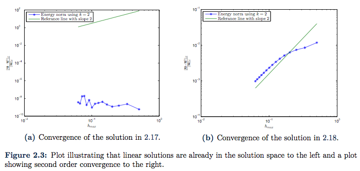
(15) $\begin{equation*} \vec{u}=\begin{bmatrix} 0\\ x\\ 0 \end{bmatrix} \end{equation*}$

which is plotted in Figure 2.1. Of course, such linear solution is already in the search space $\boldsymbol{\mathcal{S}}^h$ , so we should expect the error to be near machine epsilon. And as we can see from the convergence plot given in Figure 2.3a this is indeed that case. Here the error is more likely to originate from the approximation in quadrature rules.

Screen Shot 2014-05-03 at 20.29.12

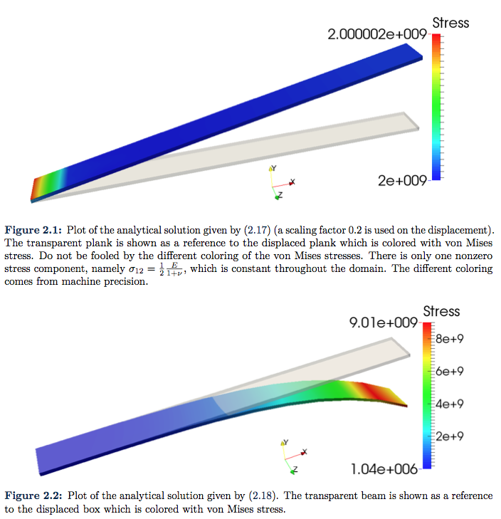
A more complex solution is given by

(16) $\begin{equation*} \vec{u}=\begin{bmatrix} \frac{1}{5}xy(2\nu^2 x^2-6\nu^2 z^2-4\nu x^2+15\nu z^2-6z^2)\\ \frac{1}{10}x^2(\nu x^2-3\nu z^2-2x^2+6z^2)\\ -\frac{3}{5}x^2 yz(\nu-2) \end{bmatrix}. \end{equation*}$

The plot of the solution is shown in Figure 2.2. The analysis is done with second order NURBS, so since the analytic solution has a third order polynomial in the $x$ direction, the solution is not in the search space $\boldsymbol{\mathcal{S}}^h$ . The convergence plot is presented in Figure 2.3b. The order of convergence is not impressive in the beginning, but it get’s closer to the expected second order of convergence as the element size get’s smaller. This is probably due to the constant $C$ , which we shall present evidence for in the next case.

Screen Shot 2014-05-03 at 20.30.31

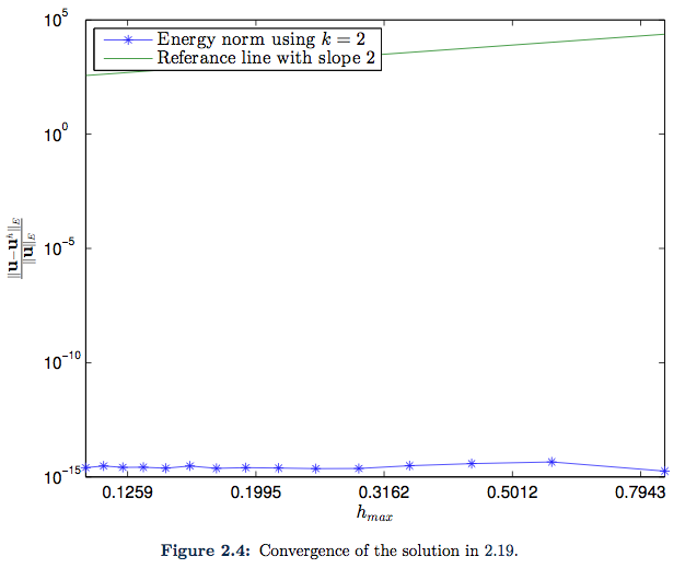
A more regular domain would be to choose $w_x=w_y=w_z=1$ , i.e. a cube. All though we have not presented so much theory on the case $\vec{f}\neq\textbf{0}$ we shall present this case on the remaining three cases. For simplicity we construct the solution such that they are zero on the boundary of the cube. That is, we only have homogeneous Dirichlet boundary. Consider the solution

(17) $\begin{equation*} \vec{u}=\begin{bmatrix} x(x-w_x)y(y-w_y)z(z-w_z)\\ x(x-w_x)y(y-w_y)z(z-w_z)\\ x(x-w_x)y(y-w_y)z(z-w_z) \end{bmatrix}. \end{equation*}$

It does indeed satisfy the conditions with a rather ugly resulting function $\vec{f}$ (the expression for this function is in fact so complex that we do not even bother to include it in the appendix). Once again, since this solution only has degree two for each polynomial in each of the spatial direction, the solution is thus an element in the search space $\boldsymbol{\mathcal{S}}^h$ , so we should expect the error to be close to machine epsilon again. As we can see from Figure 2.4 this is indeed the case.

Screen Shot 2014-05-03 at 20.30.37

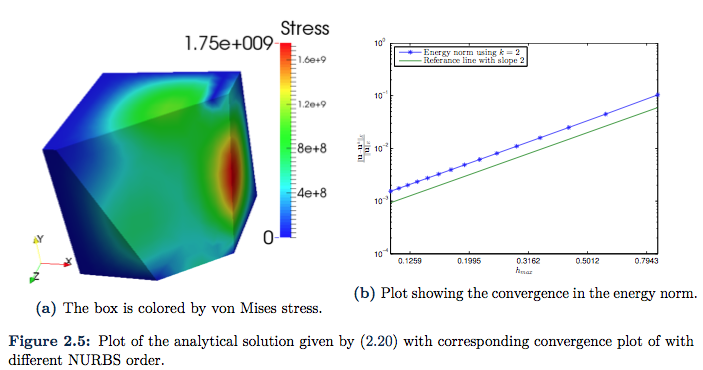
By multiplying the solution in 17 by another factor $x$ ,

(18) $\begin{equation*} \vec{u}=\begin{bmatrix} x^2(x-w_x)y(y-w_y)z(z-w_z)\\ x^2(x-w_x)y(y-w_y)z(z-w_z)\\ x^2(x-w_x)y(y-w_y)z(z-w_z) \end{bmatrix}, \end{equation*}$

we get a solution which should not be in the search space $\boldsymbol{\mathcal{S}}^h$ . The condition on the boundary does of course still hold, but now we have an even more complex function $\vec{f}$ . The displacement of the cube is not so illustrative, rather, we cut of a part of the cube such that we can see the von Mises stress at a plane inside the cube as well. This plot is given in Figure 2.5a. The convergence plot is given in Figure 2.5b, and we here observe instantaneously convergence of second order.

Screen Shot 2014-05-03 at 20.30.43

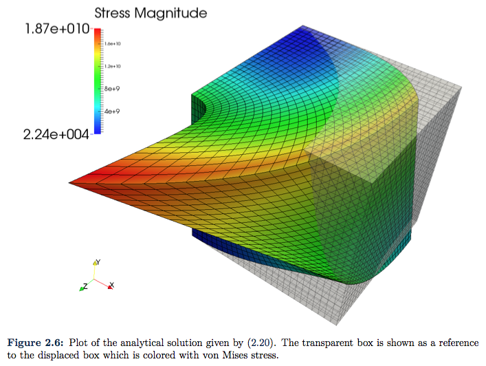
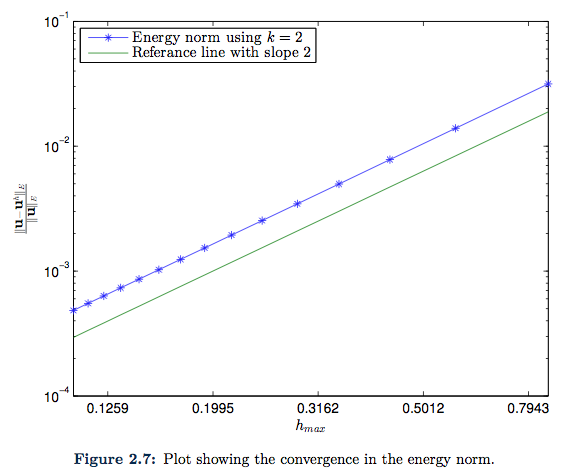
The finale example is presented just to illustrate that we have the same type of convergence when Neumann boundary condition is implemented. We plot the same analytic function in \eqref{Eq:secondAnalyticalSolution}, but here we choose $w_x=w_y=w_z=1$ . The resulting plots are given in Figure 2.6 and Figure 2.7.

Screen Shot 2014-05-03 at 20.30.57

Screen Shot 2014-05-03 at 20.31.07

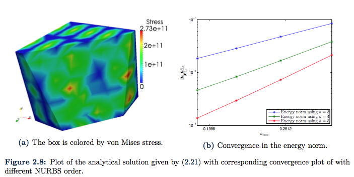
All of the discussed solutions have been polynomial solution, and whould thus potentially be in the solution space $\boldsymbol{\mathcal{S}}^h$ if we elevate the order of the NURBS. Thus, the solutions presented so far does not fit so much for analysis on the order elevation of NURBS. A trigonometric solution given by

(19) $\begin{equation*} \vec{u}=\begin{bmatrix} \sin\left(\frac{4\pi x}{w_x}\right)\sin\left(\frac{4\pi y}{w_y}\right)\sin\left(\frac{4\pi z}{w_z}\right)\\ \sin\left(\frac{4\pi x}{w_x}\right)\sin\left(\frac{4\pi y}{w_y}\right)\sin\left(\frac{4\pi z}{w_z}\right)\\ \sin\left(\frac{4\pi x}{w_x}\right)\sin\left(\frac{4\pi y}{w_y}\right)\sin\left(\frac{4\pi z}{w_z}\right) \end{bmatrix}, \end{equation*}$

will also satisfy homogeneous Dirichlet boundary conditions at the boundary. The resulting plots are given in Figure 2.8a and Figure 2.8b. In the convergence plot, we illustrate the different convergence rates by eleviating the NURBS order. It should be noted that the convergence is slightly better than $h^k$ .

Screen Shot 2014-05-03 at 20.31.13